One of the cornerstones of the seemingly weekly advancements in AI research and applications is the transformer architecture, introduced in Attention Is All You Need by Vaswani, et al in 2017. I felt the magic for myself last year when I tried out Andrej Karpathy’s nanoGPT project and was able to train a character-level language model on my Mac within minutes, and saw reasonable-looking text being produced. I wanted to try my hand at writing a transformer from scratch. After some ramping-up in machine learning (see my previous posts), I’ve finally accomplished that. Check out this notebook for a PyTorch implementation of a decoder-only transformer. To guide the development with a concrete problem to solve, I train on the same subset of the works of Shakespeare that Karpathy used for his character-level model, but use the Byte-Pair Encoding tokenizer used for GPT-2. I referenced ARENA 3.0 for some code and also found Jacob Hilton’s deep learning curriculum chapter on Transformers helpful and walk through his first-principle questions below.

Transformer Overview

Transformer models have been massively popular in the last few years and have been the go-to architecture for working with sequence data like text. Large language models (LLMs) such as the GPT series from OpenAI are all based on the transformer architecture. The core innovation behind transformers is an attention mechanism that allows the model to flexibly focus on different parts of the input sequence when producing each output element.

The original transformer model described by Vaswani, et al employed an encoder-decoder structure, but replaced RNNs with stacked self-attention and feedforward layers in the encoder and decoder. RNNs process data sequentially, whereas transformers are able to be parallelized through their unique self-attention design.

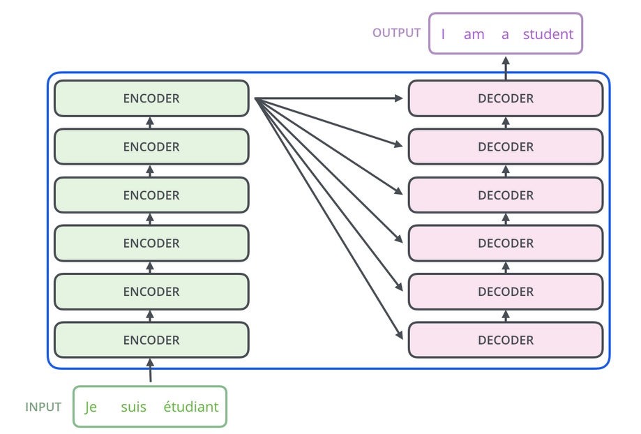seq2seq language translation diagram from The Illustrated Transformer

In the encoder, each position attends to all other positions in the input sequence to compute representations capturing their relationships. The decoder then attends to these encoded representations and previous output tokens to generate the output sequence one element at a time.

The encoder-decoder design is useful for sequence-to-sequence (seq2seq) tasks like translating text from one language to another. However, other NLP and multimodal tasks do not necessarily need a translation component, and can be architected as encoder-only or decoder-only.

Encoder-only models are not autoregressive. Instead, a latent representation of an input is captured and a classification task can be performed. BERT (Bidirectional Encoder Representations from Transformers) is an example of an encoder-only model.

In contrast, GPT is a decoder-only model, and leverages causal/unidirectional self-attention over previous tokens.

Transformer architectures have been remarkably successful and their capabilities seem to follow scaling laws as more training data, model size, and compute is applied. While initially focused on text, they are also being extended to other domains like computer vision and multimodal data.

Transformer Fundamentals

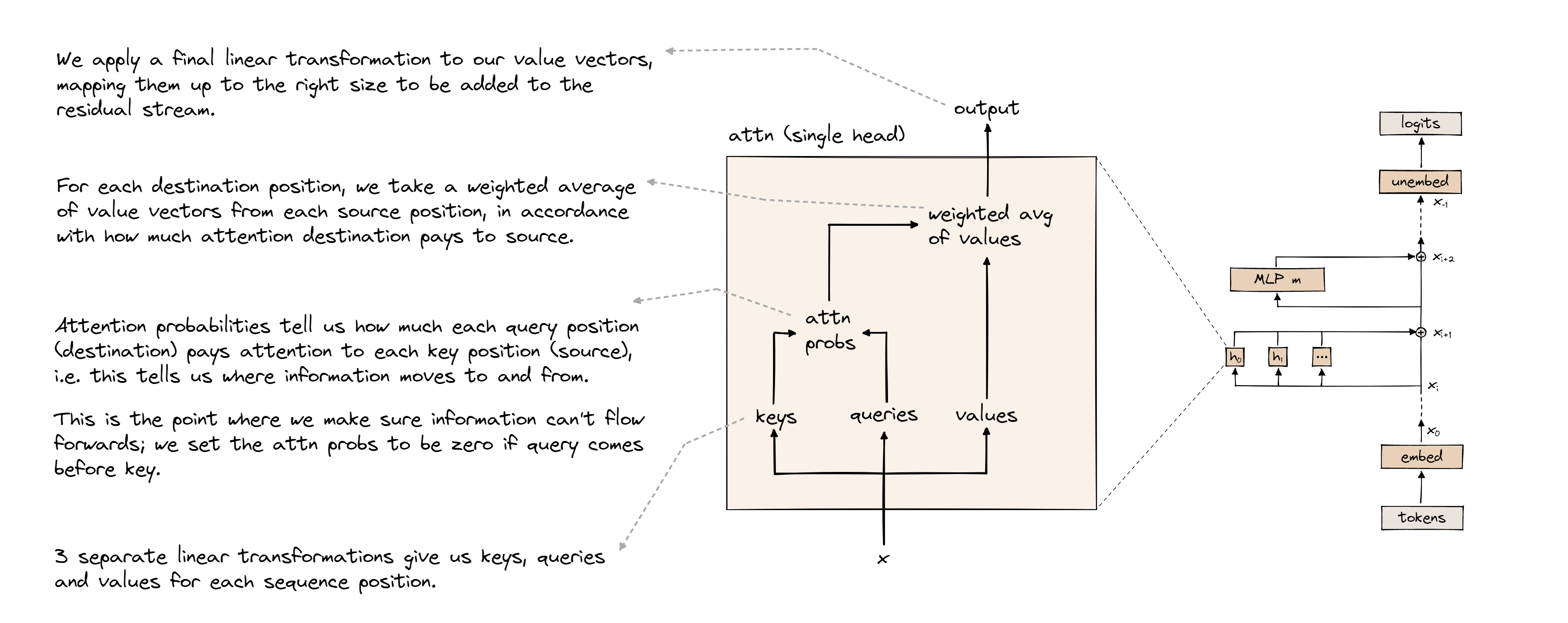Attention diagram from ARENA 3.0

What is different architecturally from the Transformer, vs a normal RNN, like an LSTM? (Specifically, how are recurrence and time managed?)

RNNs recurrently use the same blocks once per token, updating a hidden state to bring in context from previous tokens. Transformers avoid the recurrence and enjoy shared context by letting each token attend to all other tokens. However, while “time” is implicit in the sequence ordering of tokens to an RNN, attention is independent of ordering. So in order to bring in the notion of “time”, transformers explicitly add a position embedding to the embedding of its input. This allows transformers to process input data in parallel whereas RNNs are constrained to process serially.

Attention is defined as, $Attention(Q,K,V) = softmax(\frac{QK^T}{\sqrt(d_k)})V$. What are the dimensions for Q, K, and V? Why do we use this setup? What other combinations could we do with (Q,K) that also output weights?

The dimensions for Q and K are {batch_size, seq_len, n_heads, d_k}. The dimensions for V are {batch_size, seq_len, n_heads, d_v}. Notably, the last dimensions are $d_k$ and $d_v$ instead of $d_{model}$ so that the model can leverage multi-head attention instead of a single attention function. With multi-head attention, the model can jointly attend to different information in each head. Then the weighted sums (based on attention scores) of values are concatenated and reprojected into $d_{model}$. Other ways to combine (Q,K) mentioned in the original paper include additive attention and dot product attention (whereas the described self-attention is “scaled dot product attention.” The scaling factor acts as a normalization factor for longer sequences.)

Are the dense layers different at each multi-head attention block? Why or why not?

Yes each block has different dense layers so that they can learn different representations and identify unique important information.

Why do we have so many skip connections, especially connecting the input of an attention function to the output? Intuitively, what if we didn’t?

The skip connections allow for the model to have a “residual stream”, going straight from the input to the output. The residual stream allows the model to only learn modifications to the input, which is easier than having to make each layer of the model learn a larger update to get from input to output.

Causal Self-Attention Implementation

In a decoder-only transformer model, causal self-attention is employed. While during inference it’s inherently the case that future tokens are not attended to simply because they haven’t yet been generated, we need to be careful about which tokens can be attended to during training. In the training phase, predictions for every token’s next token are generated simultaneously. It’s important that for a token A in the middle of the input sequence, none of the tokens that come after A in the sequence are referenced for making a prediction about the token that should follow A.

Here’s the implementation of the attention mechanism that can be found in the accompanying notebook.

class Attention(nn.Module):
  def __init__(self, cfg):
    super().__init__()
    self.cfg = cfg
    self.W_Q = nn.Parameter(torch.empty(cfg.n_heads, cfg.d_model, cfg.d_head))
    self.W_K = nn.Parameter(torch.empty(cfg.n_heads, cfg.d_model, cfg.d_head))
    self.W_V = nn.Parameter(torch.empty(cfg.n_heads, cfg.d_model, cfg.d_head))
    self.W_O = nn.Parameter(torch.empty(cfg.n_heads, cfg.d_head, cfg.d_model))
    self.b_Q = nn.Parameter(torch.zeros(cfg.n_heads, cfg.d_head))
    self.b_K = nn.Parameter(torch.zeros(cfg.n_heads, cfg.d_head))
    self.b_V = nn.Parameter(torch.zeros(cfg.n_heads, cfg.d_head))
    self.b_O = nn.Parameter(torch.zeros(cfg.d_model))
    self.register_buffer("IGNORE", torch.tensor(-1e5, dtype=torch.float32, device=device))

  def forward(self, x):
    Q = einops.einsum(x, self.W_Q,
                      'batch pos d_model, n_heads d_model d_head -> \
                      batch pos n_heads d_head') + self.b_Q
    K = einops.einsum(x, self.W_K,
                      'batch pos d_model, n_heads d_model d_head -> \
                      batch pos n_heads d_head') + self.b_K
    V = einops.einsum(x, self.W_V,
                      'batch pos d_model, n_heads d_model d_head -> \
                      batch pos n_heads d_head') + self.b_V

    # Calculate attention scores, then scale and mask
    attn_scores = einops.einsum(Q, K,
                                'batch pos_Q n_heads d_head, \
                                batch pos_K n_heads d_head -> \
                                batch n_heads pos_Q pos_K')

    attn_scores_masked = self.apply_causal_mask(attn_scores / self.cfg.d_head ** 0.5)

    attn_pattern = attn_scores_masked.softmax(-1)

    # Take weighted sum of values based on attention pattern
    v_sum = einops.einsum(attn_pattern, V,
                          'batch n_heads pos_Q pos_K, \
                          batch pos_K n_heads d_head -> \
                          batch pos_Q n_heads d_head')

    # Calculate output
    return einops.einsum(v_sum, self.W_O,
                         'batch pos_Q n_heads d_head, \
                         n_heads d_head d_model -> \
                         batch pos_Q d_model') + self.b_O

  def apply_causal_mask(self, attention_scores):
    ones = torch.ones(attention_scores.shape[-2], attention_scores.shape[-1],
		      device=attention_scores.device)
    mask = torch.triu(ones, diagonal=1).bool()

    return attention_scores.masked_fill_(mask, self.IGNORE)

Toy example: Reversing a random string

One way to validate our implementation of causal self-attention is by seeing if a trained model is able to reverse a random string but unable to predict the next tokens as the string is revealed.

Let the sequence of tokens be random integers from 0 to 99 such that the vocab size is 100. We randomly generate sequences of length 16, with the second half mirroring the first. The model should be able to predict the second half of the sequence, but not the first.

In language models, we typically want to compare the predicted log-probabilities with the actual next token in the sequence. We exclude the log-probabilities for the last token in each sequence, as we don’t have a “next token” to compare it with.

Since we start with randomized weights and randomly generated data, we should expect the loss to start at a particular value, and be lower bounded by another value.

Since the integers in the sequence can take on any value from 0 to 99 with equal probability, an untrained model should have average loss around $-ln(\frac{1}{100}) ≈ 4.6$.

A trained model should be able to accurately predict the second half of each sequence, so the average loss for predicting a sequence of length $16$ should converge to $-ln(\frac{1}{100}) * \frac{7}{15} + -ln(\frac{1}{1}) * \frac{8}{15} \approx 2.149$.

The $15$ in the denominator comes from discarding the last prediction in the sequence since it has nothing to match with. The first $7$ elements of the sequence should not be predictable, but the 8th-15th prediction should match with the 1st-8th elements of the input.

After training for a few minutes with a single T4 GPU, we find that our training and validation loss do indeed converge to $2.149$. We also find that the second half of a test sequence is predicted accurately while the first half remains incorrect random guesses.

What if there’s no positional embedding?

Learning to successfully reverse a random string is highly dependent on the position of each token in a sequence. Because they are randomly generated, there is no relationship between adjacent tokens, and the only relevant relationship is position relative to the end of the first half of the sequence.

What happens if we don’t use a position embedding? Is the model still able to learn?

Training under the same conditions as before, but without adding a positional embedding to the input embedding in the architecture, we find that the model is still able to learn the mirror pattern. It’s more difficult to learn without the positional embedding, as evidenced by the slower rate of convergence, but somehow the model is still able to learn to represent the positions. Interestingly, we also see that for the first half, the model also started to learn to predict the last integer it saw in its input sequence, even though there was no particular steering toward that.

Further interpretability study would be necessary to pinpoint what’s happening at the circuits-level of the architecture to achieve this result. However, I suspect it’s because this toy problem is primarily about doing lookups based on a single position and the residual stream has enough bandwidth to carry the learned position information without an explicit positional embedding.

Shakespeare

Alright, now let’s try to learn some structure and style by training a model to generate Shakespeare-like text. We use a 1.1 MB file provided by Karpathy that contains a large subset of Shakespeare’s work as our dataset. We also leverage tiktoken, an open-source BPE tokenizer library from OpenAI, with a GPT-2 tokenizer. The tokenizer has a vocab size of 50,257.

We don’t need to get fancy with our transformer. A simple 2-layer model with a model width of 256 gets us decent-looking results after only a few minutes of training on a T4 GPU on Colab.

The result is mostly nonsensical but is obviously Shakespeare-esque in style.

With a prompt of

 O Romeo, Romeo, wherefore art thou Romeo?

the model generates

OXFORD:
King Edward's name;

'Twixt thy head and clas in the viewless dasticite,
From thy foul mouth the world: I hadst not what they
That thou seest it pass'd, but only I
Wherein thy suffering thus blest to heaven.
My revenge it in the female seas:
Thou art a mother of thy mother's face,
Or thou hast not but thy brother's son,
And heap thyself old grandsire's eye
Than curse thy valourers breast.

KING LEWIS XI:
Warwick, the king, or thou art the post that word.

WARWICK:
Nay, York will to Coventry.

Nay, wilt thou not?
Thou wast thou in likeness, thou shalt come about thy horse.

EXETER:
I shall not go so, as thou

Sampling for output generation

The generated text above is the result of sampling the autoregressively generated logits a particular way. There exists many possible ways to sample for outputs.

One possible way is greedy search: always choosing the highest probability token. Given the same input, the model will always generate the same output.

Another way is to randomly sample from the distribution defined by the generated logit vector (which is of the size of the vocab size).

Yet another way is to take the top k most probable tokens in the generated logit vector, reweight them with softmax, then sample from that distribution.

The “temperature” of the softmax during sampling can also be played with. A temperature of 1 is default. Lowering the temperature makes the model more confident in its predictions, and therefore lower variance in its output. A Higher temperature results in higher variance.

A more detailed treatment of sampling for output generation can be found here.

Interpretability: What’s actually happening inside a transformer?

I’m curious about transformer internals and being able to identify interpretable “circuits” within a model. I won’t go too much into this topic in this post, as there remains much to learn, but some intuition is described in the following references:

Andrej Karpathy also gives some intuition about the purpose of various architectural details in his youtube walkthrough “Let’s build GPT: from scratch, in code, spelled out”.

On attention as a generalized convolution from ARENA 3.0:

“We can think of attention as a kind of generalized convolution. Standard convolution layers work by imposing a “prior of locality”, i.e. the assumption that pixels which are close together are more likely to share information. Although language has some locality (two words next to each other are more likely to share information than two words 100 tokens apart), the picture is a lot more nuanced, because which tokens are relevant to which others depends on the context of the sentence. For instance, in the sentence “When Mary and John went to the store, John gave a drink to Mary”, the names in this sentence are the most important tokens for predicting that the final token will be “Mary”, and this is because of the particular context of this sentence rather than the tokens’ position. Attention layers are effectively our way of saying to the transformer, “don’t impose a prior of locality, but instead develop your own algorithm to figure out which tokens are important to which other tokens in any given sequence.”

Counting parameters in a transformer

For a guide on calculating the number of parameters in a model, check out

Memory usage in a transformer

Here’s some resources on how to reduce memory usage during inference by caching the K and V matrices. In short, during training, the full input sequence is available, so self-attention can be computed in a single pass over the sequence. However, during inference, the output sequence is generated autoregressively, and a single token is added to the input each time. It’s then helpful to cache the K and V matrices and add on a single row for the new token each time.

Transformer concepts and code references

Further exercises

Train the GPT on your own dataset of choice! What other data could be fun to blabber on about? (A fun advanced suggestion if you like: train a GPT to do addition of two numbers, i.e. a+b=c. You may find it helpful to predict the digits of c in reverse order, as the typical addition algorithm (that you’re hoping it learns) would proceed right to left too. You may want to modify the data loader to simply serve random problems and skip the generation of train.bin, val.bin. You may want to mask out the loss at the input positions of a+b that just specify the problem using y=-1 in the targets (see CrossEntropyLoss ignore_index). Does your Transformer learn to add? Once you have this, swole doge project: build a calculator clone in GPT, for all of +-*/. Not an easy problem. You may need Chain of Thought traces.)
Find a dataset that is very large, so large that you can’t see a gap between train and val loss. Pretrain the transformer on this data, then initialize with that model and finetune it on tiny shakespeare with a smaller number of steps and lower learning rate. Can you obtain a lower validation loss by the use of pretraining?
Read some transformer papers and implement one additional feature or change that people seem to use. Does it improve the performance of your GPT?

Other exercises:

transformer-circuits exercises

Welcome to Henry's blog! A work in progress

About Writing Contact

Building a Transformer From Scratch

Transformer Overview

Transformer Fundamentals

Causal Self-Attention Implementation

Toy example: Reversing a random string

What if there’s no positional embedding?

Shakespeare

Sampling for output generation

Interpretability: What’s actually happening inside a transformer?

Counting parameters in a transformer

Memory usage in a transformer

Further reading

Transformer concepts and code references

Further exercises

Building a Transformer From Scratch

Transformer Overview

Transformer Fundamentals

Causal Self-Attention Implementation

Toy example: Reversing a random string

What if there’s no positional embedding?

Shakespeare

Sampling for output generation

Interpretability: What’s actually happening inside a transformer?

Counting parameters in a transformer

Memory usage in a transformer

Further reading

Transformer concepts and code references

Further exercises

You may also enjoy:

Optimizers

Building a Mini Neural Network Library: Backpropagation and Autograd