This blog post accompanies minigrad, a mini autograd engine for tensor operations and a small neural network library on top of it.

Going through a typical training loop, we would see the following steps:

1. Run input data through the model to generate logits.
2. Calculate the loss by comparing the logits with the labels via a loss function.
3. Backpropagate and calculate the gradients with a call to loss.backward().
4. Update the weights with a call to optimizer.step().
5. Zero out the gradients by calling optimizer.zero_grad().

If you’re like me, the first two steps are easy to imagine and make sense - they’re just function calls. The last two steps also make sense since we pass the model weights to the optimizer. But the backpropagation step for gradient updates needs more explanation.

How does calling loss.backward() propagate through all the layers and compute all the gradients?

By the end of this post, we should know enough to implement our own autograd engine and mini neural network library with a PyTorch-like API.

Backpropagation

Backpropagation, or reverse-mode differentiation, is a really efficient way to evaluate derivatives of a multivariable function with many variables. Depending on the number of variables, it can be multiple orders of magnitude faster than the alternative, forward-mode differentiation.

Lets use the following convex function as a lens through which to view the upcoming ideas:

$f(x,y) = 3x^2 + xy + 5y^2$

Computational Graph

We can represent a function (and its derivatives) with a computational graph of the primitive operations between function variables, like add and multiply.

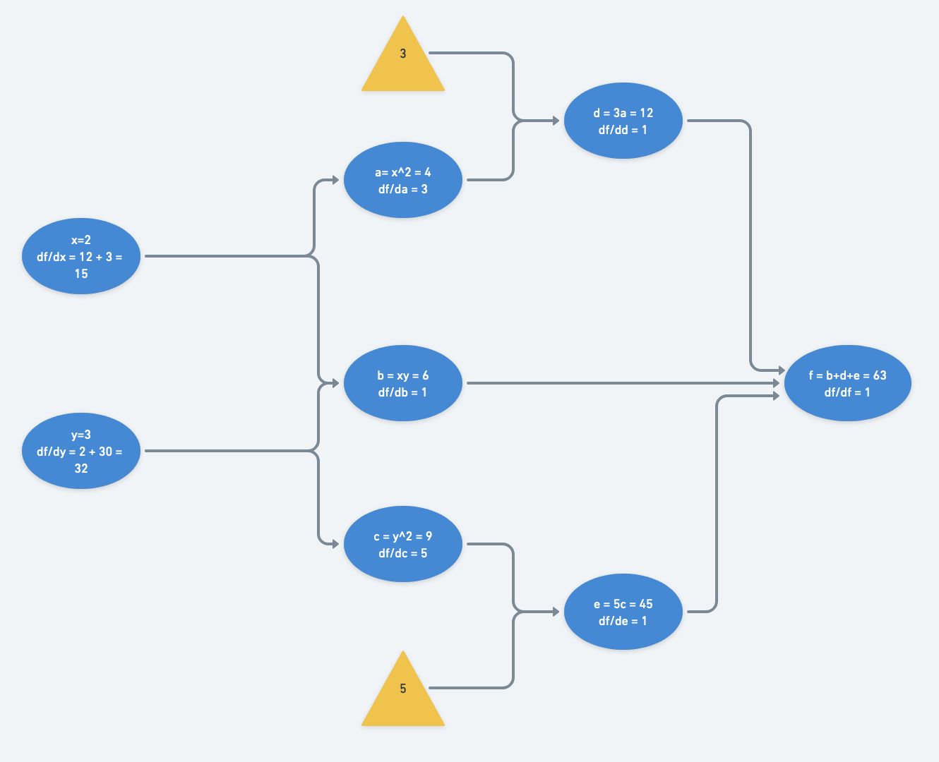
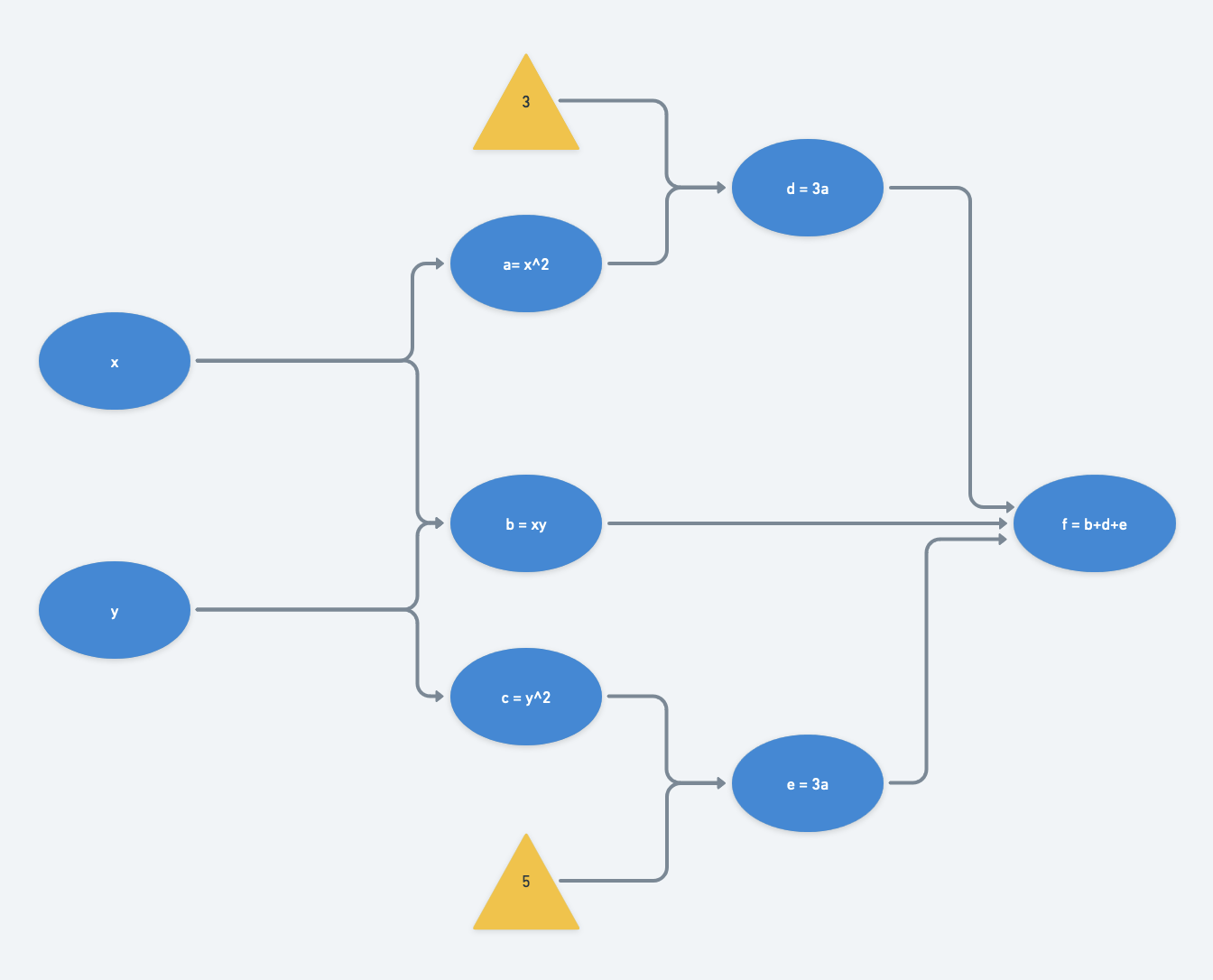
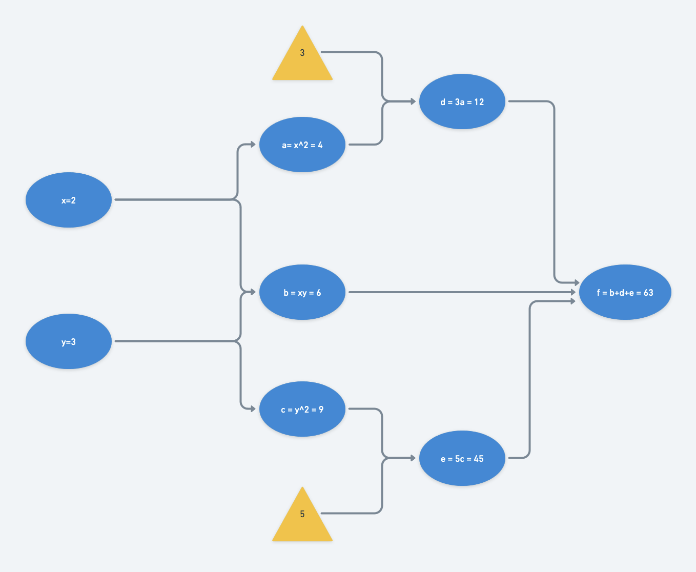
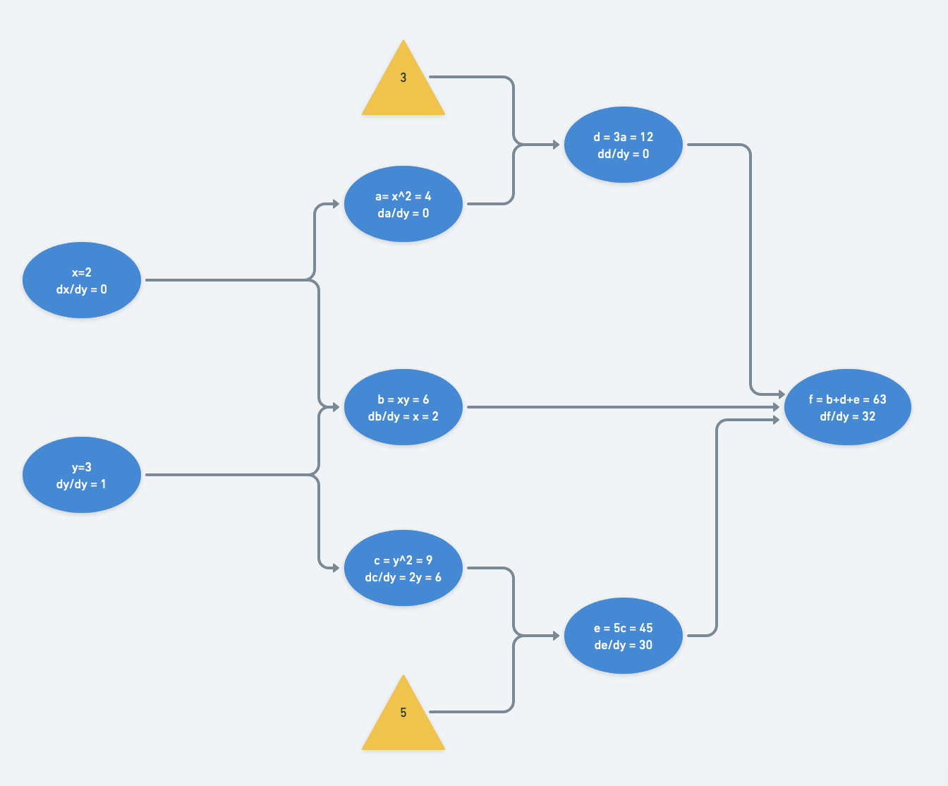
For our example function $f(x,y)$, let $a=x^2$, $b=xy$, and $c=y^2$. Then we can rewrite $f$ in terms of $a,b,c$:

$f(x,y) = f(a,b,c) = 3a + b + 5c$

Its computational graph would be, with $d=3a$ and $e=5c$:

At a particular set of inputs, say say $x=2$ and $y=3$, we can run through the computational graph from left to right (a “forward pass”) and find that $f(x=2,y=3) = 63$:

Now lets consider $f(x,y)$ as a loss function to be minimized (recall that $f(x,y)$ is convex). We want to find the optimal $(x,y)$ pair.

It can be solved by taking the partial derivatives of $f(x,y)$, setting up a system of linear equations by setting the derivatives equal to $0$, and solving for $x$ and $y$ by inverting the coefficient matrix.

However, in deep learning, we solve using iterative numerical methods, like gradient descent. At each iteration, we are at a particular $(x,y)$ pair. We check our “loss” by evaluating the function where we currently are. To improve on our loss, we evaluate our gradients where we are and take a step in the opposite direction (in vanilla gradient descent; other approaches also approximate the Hessian to influence the step direction based on function curvature).

With iterative numerical methods, there are two ways to think about traversing the computational graph for evaluating partial derivatives: forward-mode and reverse-mode differentiation.

Forward-mode differentiation

In an introduction to calculus class, we learn how to take the partial derivatives of a multivariable function with respect to each of its variables, applying the chain rule where necessary.

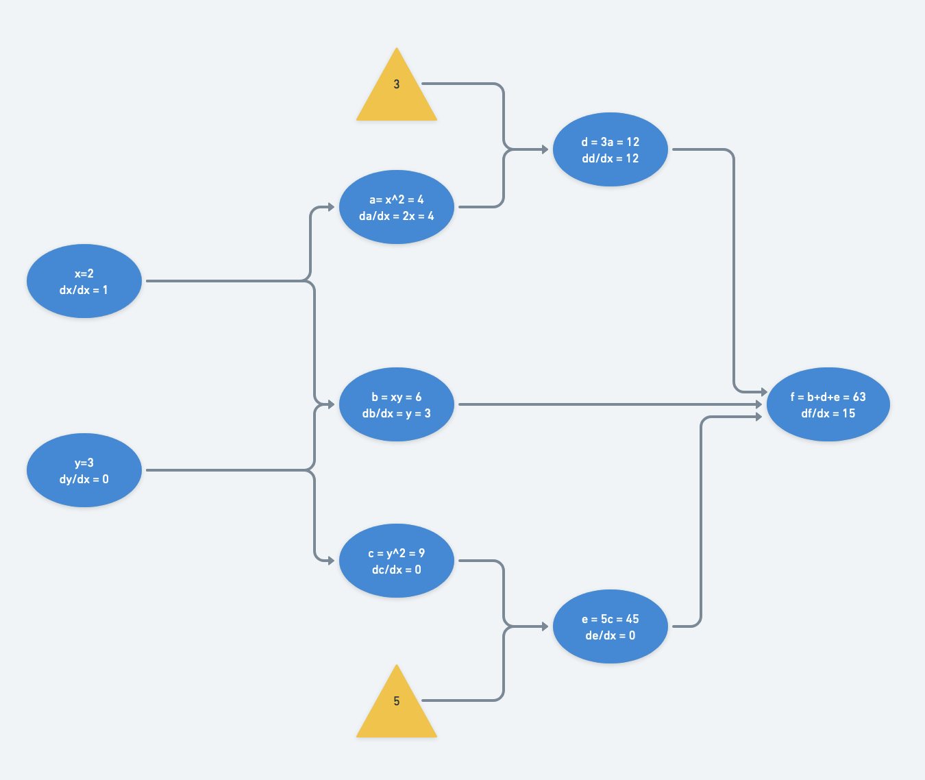
For our example function, we reproduce the substitutions here for easy reference:

$a=x^2$, $b=xy$, $c=y^2$, $d=3a$, $e=5c$, $f = d + b + e$

With forward-mode differentiation, we must calculate $\frac{df}{dx}$ and $\frac{df}{dy}$ separately.

Its partial derivatives, in forward-mode differentiation are calculated like so:

$\frac{df}{dx} = \frac{dx}{dx}(\frac{da}{dx}(\frac{dd}{da}) + \frac{db}{dx}) + \frac{dy}{dx}(\frac{db}{dy} + \frac{dc}{dy}(\frac{de}{dc})) $

$= 1 \cdot (2x \cdot 3 + y) + 0 \cdot (x + 2y \cdot 5) $

$= 6x + y$

$\frac{df}{dy} = \frac{dx}{dy}(\frac{da}{dx}(\frac{dd}{da}) + \frac{db}{dx}) + \frac{dy}{dy}(\frac{db}{dy} + \frac{dc}{dy}(\frac{de}{dc})) $

$= 0 \cdot (2x \cdot 3 + y) + 1 \cdot (x + 2y \cdot 5) $

$= x + 10y$

However, rather than plugging in the input values once the partial derivative symbolic expressions have been computed, the derivative with respect to each node is evaluated and propagated forward in the computational graph. The former would require much more memory to hold onto each node’s symbolic expressions.

The computational graph is traversed twice from left to right: once for derivatives with respect to $x$ and once for those with respect to $y$.

With just two inputs, this isn’t so bad. However it becomes much more computationally expensive when the number of inputs increases. The magnitude of increase in computational complexity scales with the number of paths from inputs to outputs. Reverse-mode differentiation to the rescue.

Reverse-mode differentiation

When performing reverse-mode differentiation, we propagate (evaluated) derivatives backwards from the outputs to the inputs.

In symbolic form, the partial derivatives expanded out would be:

$\frac{df}{dx} = \frac{df}{df}\frac{df}{dd}\frac{dd}{da}\frac{da}{dx} + \frac{df}{df}\frac{df}{db}\frac{db}{dx} + \frac{df}{df}\frac{df}{de}\frac{de}{dc}\frac{dc}{dx} $

$= 1 \cdot 1 \cdot 3 \cdot (2x) + 1 \cdot 1 \cdot y + 1 \cdot 1 \cdot 5 \cdot 0 $

$ = 6x + y$

$\frac{df}{dy} = \frac{df}{df}\frac{df}{dd}\frac{dd}{da}\frac{da}{dy} + \frac{df}{df}\frac{df}{db}\frac{db}{dy} + \frac{df}{df}\frac{df}{de}\frac{de}{dc}\frac{dc}{dy} $

$= 1 \cdot 1 \cdot 3 \cdot 0 + 1 \cdot 1 \cdot x + 1 \cdot 1 \cdot 5 \cdot (2y) $

$ = x + 10y$

The decrease in number of operations compared with forward-mode differentiation is most obvious when looking at the computational graph after gradients are calculated and accumulated.

Notice only a single pass backwards is necessary to compute the gradient with respect to each node.

Batch Backpropagation

Typically when training a model, we don’t calculate gradients one example at a time; we use minibatches of examples. So how does updating the computational graph work when we have multiple data points per node and we need to propagate the evaluated gradients?

Well, instead of maintaining a scalar for each node’s output and gradient, we maintain matrices instead. The gradients from each example would be averaged together so that the training is invariant to batch size.

A concrete example would be a linear layer followed by a MSE loss like we explored in a previous post. Let’s say we’re doing linear regression, working with a minibatch of N=64 example 2D points, with $X$ as the inputs and $Y$ as the labels. $X$ has shape $N \times 2$ (column of x values and column of ones). $Y$ has shape $N \times 1$. $W$ has shape $2 \times 1$. Then $P = XW$ has shape $N \times 1$, and $L$ is a scalar.

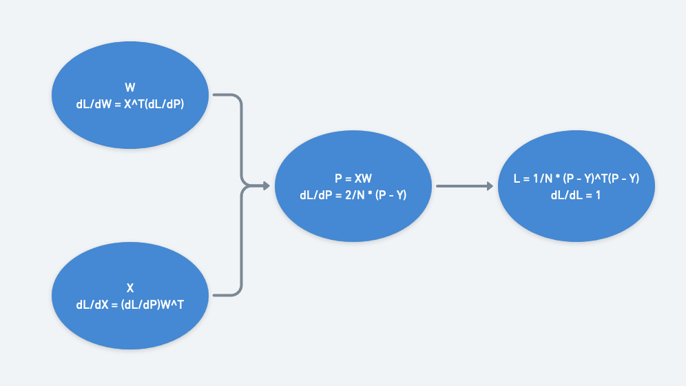
We can work backwards from the loss node of the computational graph. Since the loss is a scalar, all its gradients with respect to each node’s output should take on the shape of the node’s output. $\frac{dL}{dP}$ has shape $N \times 1$, $\frac{dL}{dW}$ has shape $2 \times 1$, and $\frac{dL}{dX}$ has shape $N \times 2$.

Note: Since we care only about updating the weights, we could have specified that we don’t need gradients calculated with respect to $X$.

Here’s $\frac{dL}{dW}$ expanded out:

\[\frac{dL}{dW} = X^T \frac{dL}{dP} =\frac{2}{N} \begin{pmatrix} x_1 & x_2 & \cdots & x_N \\\ 1 & 1 & \cdots & 1\\\ \end{pmatrix} \begin{pmatrix} p_1 - y_1 \\\ p_2 - y_2 \\\ ... \\\ p_N - y_N \\\ \end{pmatrix}\] \[= \frac{2}{N} \begin{pmatrix} x_1 \cdot (p_1 - y_1) + \cdots + x_N \cdot (p_N - y_N) \\\ (p_1 - y_1) + \cdots + (p_N - y_N) \\\ \end{pmatrix}\]

Notice each of the two gradient values comes from the mean of earlier gradients.

Computational Graph View of an MLP

When we see a typical textbook version of an MLP, it is drawn pretty similarly to what we see below. We have M input features, two hidden layers with J and K features respectively, and an output layer with N features.

So how does this view of an MLP connect with the computational graphs that we just introduced?

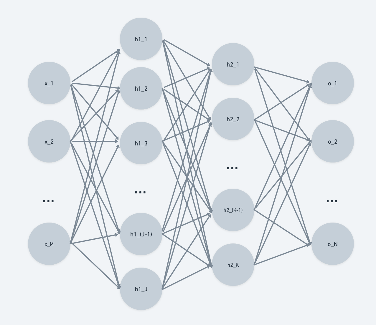
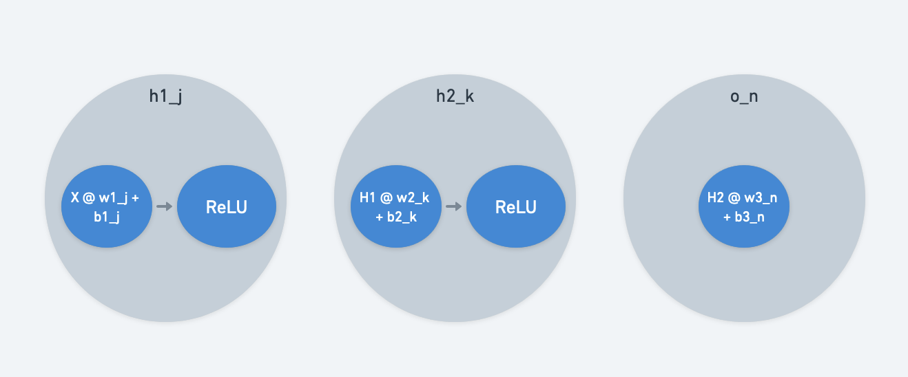
The computational graph is a low-level view of operations. When we introduced computational graph nodes, we let them separately represent model inputs, weights, and operations.

To make those ideas match with the MLP diagram, we allow each MLP neuron to combine weights and operations on its inputs. The MLP neural network view is a mid-level view.

We typically think of neural nets in terms of layers - this would be a high-level view, with the 2-layer MLP containing input layer $X$, hidden layers $H1$ and $H2$, and output layer $O$. Each layer is composed of a stack of neurons.

Summary

In summary, backpropagation can be thought of as applying the chain rule backwards on a computational graph and evaluating the gradients at the current weight values. The chain rule is applied backward (reverse-mode differentiation) because for a typical neural network with more inputs than outputs, it’s much more efficient to calculate the derivative of the loss with respect to every node than to calculate the derivative of every node with respect to every input (forward-mode differentiation).

Other Resources

• For a similar popular explanation of backpropagation with computational graphs, check out Calculus on Computational Graphs: Backpropagation by Chris Olah.
• Further math and intuition behind backpropagation through a linear layer is worked through in detail in this CS231n handout.
• Other work connects math and code for batch backpropagation, similar to this previous post.

Autograd

Now that we have a handle on the mechanics of backpropagation, lets get back to the question of how calling loss.backward() propagates through all the layers and compute all the gradients.

With a computational graph concept, we can manually write a forward and backward pass through the nodes of the graph. This works fine for a small network, but it can become really cumbersome for a larger, deeper network.

We need to add on some more ideas necessary to automate the gradient calculations with a single call to the loss Tensor.

Tensor objects and building a computational graph

Each node of our computational graph doesn’t just output an out array. A node can also contain

• the forward function used to compute out based on its inputs arrays
• its inputs arrays used for evaluating gradients.
• where the inputs came from, or the node’s parents.
• any keyword args to apply to the forward function, or kwargs.
• requires_grad boolean for whether or not a gradient needs to be computed for the node.
• the evaluated gradient of the loss with respect to the node’s out .

We choose to construct the computational graph during the forward pass and hold the above information in the forward output of a node: A Tensor object.

When considering a neural network layer, we can think of it as being composed of a leaf node that holds the weights and another node that applies the weights to the inputs to the layer.

Topological Ordering

In our section on backpropagation, we heavily used the idea of a computational graph. Recall that in order to evaluate the gradient of the loss with respect to each node, we needed all preceding gradients to be calculated.

But how do we make sure we calculate all preceding gradients first?

We need a topological sort of the computational graph nodes.

Topological sorting operates on directed acyclic graphs (DAGs) to visit each node once. A topological sort returns an ordered list of nodes to evaluate.

“backward” functions

For a forward function, we need a corresponding backward function (or multiple backwards in the case of multiple inputs). Additionally, we need a way to automatically get the backwards associated with the forward functions.

There are many ways to associate functions. PyTorch, for example, maintains a derivatives.yaml file of derivatives for each forward function.

“No-Grad” Context Manager

Sometimes we don’t want to build or add on to a computational graph. Examples include when weight updates are being performed after the backward pass and when evaluating validation/test data. A context manager is needed to switch between the two modalities of needing vs not needing gradients to be computed.

Other resources

• Overview of PyTorch Autograd Engine
• [ARENA 3.0: Backprop(]https://arena3-chapter0-fundamentals.streamlit.app/[0.4]_Backprop)
• PyTorch Examples - Justin Johnson

A mini autograd engine and neural network library

If we put together all the autograd concepts, we can build an autograd engine. The bulk of the work is in defining all the functions to support. Each function would need an implementation for propagating the evaluated gradient with respect to each of its inputs.

Once an autograd engine is built, there are not too many more steps needed to build a neural network library on top of it.

A nn.Parameter simply wraps a Tensor and sets its requires_grad flag to True. A nn.Module needs to be implemented to store state information in the form of other nn.Modules and nn.Parameters.

Then any custom layers, like nn.Linear or nn.ReLU, can easily be defined on top of nn.Module, with an implementation of their forward pass. The backward is implicitly defined since we’ve specified the gradients of all the primitive operations that make up the forward.

An optimizer such as SGD can be defined which takes in the parameters to update. A stateless loss function is all that’s left to make a neural network library that can train.

Check out minigrad for implementation details.